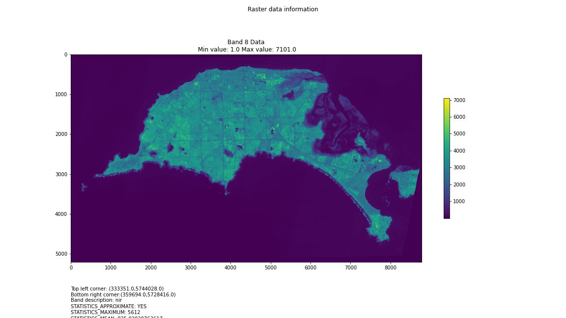
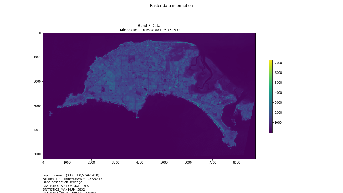
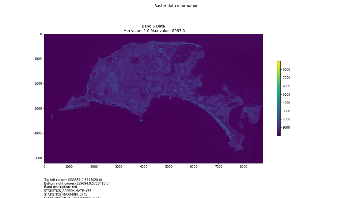
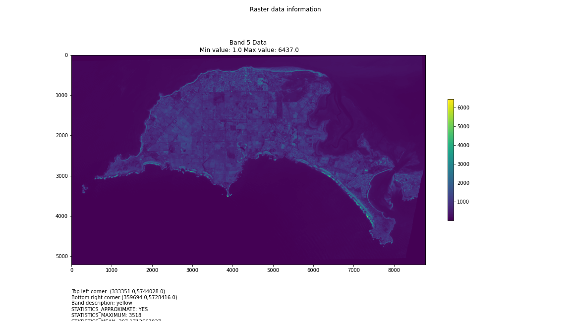
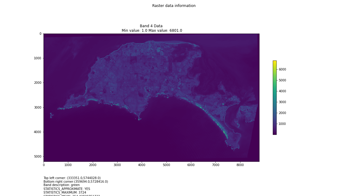
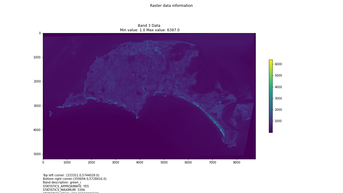
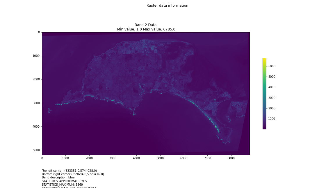
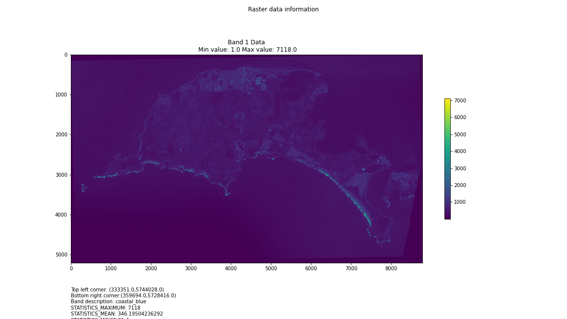
One objective (amongst many) that Chris and I have identified is to first start off looking at islands. The reason behind this is simple: an island presents a defined and constrained geographic area – not too big, not too small (depending on the island, of course) – and I’ve had a lot of recent experience working with island data on my recent Macquarie Island project with my colleague Dr Gina Moore. It provides some practical limits to the amount of data we have to work with, whilst engaging many of the technical issues one might have to address.
With this in mind, we’ve started looking a Philip Island (near Melbourne, Victoria) and Kangaroo Island (South Australia). Both fall under a number of satellite paths, from which we can isolate multispectral and hyperspectral data. I’ll add some details about these in a later post – as there are clearly issues around access and rights that need to be absorbed, explored and understood.
For a first attempt, here is a google colab script for looking at some Philip Island data from the XXX Satellite:
# Import necessary librariesimport osfrom osgeo import gdal, gdal_arrayfrom google.colab import driveimport numpy as npimport matplotlib.pyplot as plt# Mount Google Drivedrive.mount('/content/drive')#this will ask for permissions - you will need to login through your google account in a pop-up window# Open the multispectral GeoTIFF file#set the file path to the folder with the relevant data in it on your google drive (mount this first via the panel to the left of this one - it is called 'drive' and appears as a folder)file_path = '/content/drive/MyDrive/DATA/XXX_multispectral.tif'#set a variable for your path and the file you opensrc_ds = gdal.Open(file_path)#use gdal to get some characteristics of the data in the fileprint("Projection: ", src_ds.GetProjection()) # get projectionprint("Columns:", src_ds.RasterXSize) # number of columnsprint("Rows:", src_ds.RasterYSize) # number of rowsprint("Band count:", src_ds.RasterCount) # number of bandsprint("GeoTransform", src_ds.GetGeoTransform()) #affine transform# Use gdalinfo command to print and save information about the raster file - this is extracted from the geotiff itselfinfo = gdal.Info(file_path)print(info)if not os.path.exists("/content/drive/MyDrive/DATA/OUTPUT"): os.makedirs("/content/drive/MyDrive/DATA/OUTPUT")info_file = os.path.join("/content/drive/MyDrive/DATA/OUTPUT", "raster_info.txt")with open(info_file, "w") as f: f.write(info)# Retrieve the band count and band metadatadata_array = src_ds.GetRasterBand(1).ReadAsArray()data_array.shapeband_count = src_ds.RasterCount# Loop through each band and display in a matplotlib imagefor i in range(1, band_count+1): band = src_ds.GetRasterBand(i) minval, maxval = band.ComputeRasterMinMax() data_array = band.ReadAsArray() plt.figure(figsize=(16, 9)) plt.imshow(data_array, vmin=minval, vmax=maxval) plt.colorbar(anchor=(0, 0.3), shrink=0.5) plt.title("Band {} Data\n Min value: {} Max value: {}".format(i, minval, maxval)) plt.suptitle("Raster data information") band_description = band.GetDescription() metadata = band.GetMetadata_Dict() geotransform = src_ds.GetGeoTransform() top_left_x = geotransform[0] top_left_y = geotransform[3] w_e_pixel_res = geotransform[1] n_s_pixel_res = geotransform[5] x_size = src_ds.RasterXSize y_size = src_ds.RasterYSize bottom_right_x = top_left_x + (w_e_pixel_res * x_size) bottom_right_y = top_left_y + (n_s_pixel_res * y_size) coordinates = ["Top left corner: ({},{})".format(top_left_x,top_left_y),"Bottom right corner:({},{})".format(bottom_right_x,bottom_right_y)] if band_description: metadata_list = ["Band description: {}".format(band_description)] else: metadata_list = ["Band description is not available"] if metadata: metadata_list += ["{}: {}".format(k, v) for k, v in metadata.items()] else: metadata_list += ["Metadata is not available"] plt.annotate("\n".join(coordinates+metadata_list), (0,0), (0, -50), xycoords='axes fraction', textcoords='offset points', va='top') plt.savefig("/content/drive/MyDrive/DATA/OUTPUT/Band_{}_Data.png".format(i), vmin=minval, vmax=maxval) plt.show()
This works well enough for a plot – but it’s interesting (a debate) – whether it is best/easiest to use GDAL or the rasterio Mapbox wrapper. Tests will tell. And there is Pandas too. They all have pros and cons. Try it yourself and let us know,
I’m looking into ways of sharing the colabs more directly for those who are interested – that’s the whole point.

