Tag Archives: colab

Visualising Philip Island

One objective (amongst many) that Chris and I have identified is to first start off looking at islands. The reason behind this is simple: an island presents a defined and constrained geographic area – not too big, not too small (depending on the island, of course) – and I’ve had a lot of recent experience working with island data on my recent Macquarie Island project with my colleague Dr Gina Moore. It provides some practical limits to the amount of data we have to work with, whilst engaging many of the technical issues one might have to address.

With this in mind, we’ve started looking a Philip Island (near Melbourne, Victoria) and Kangaroo Island (South Australia). Both fall under a number of satellite paths, from which we can isolate multispectral and hyperspectral data. I’ll add some details about these in a later post – as there are clearly issues around access and rights that need to be absorbed, explored and understood.

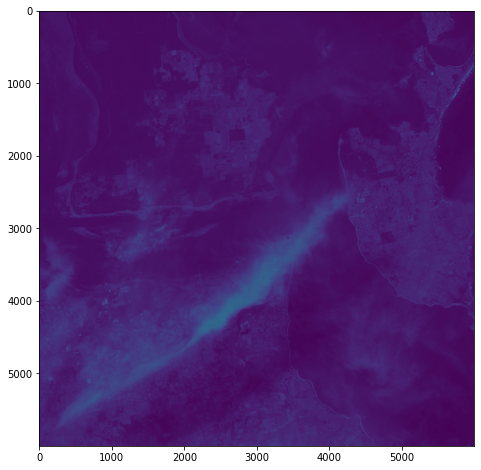
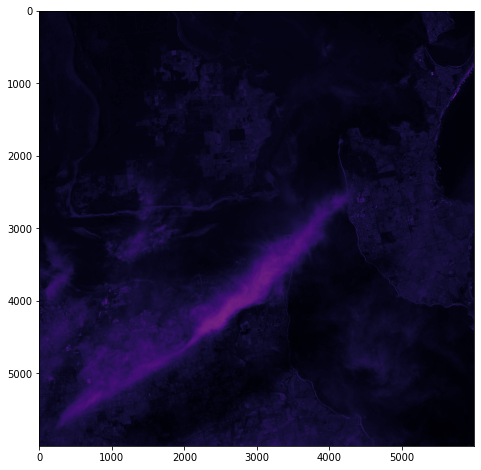
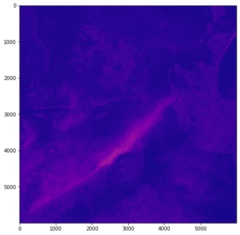
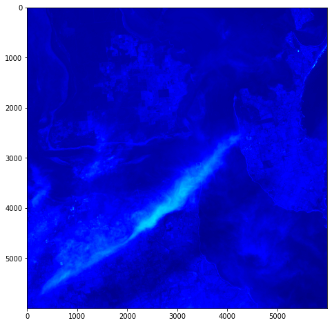
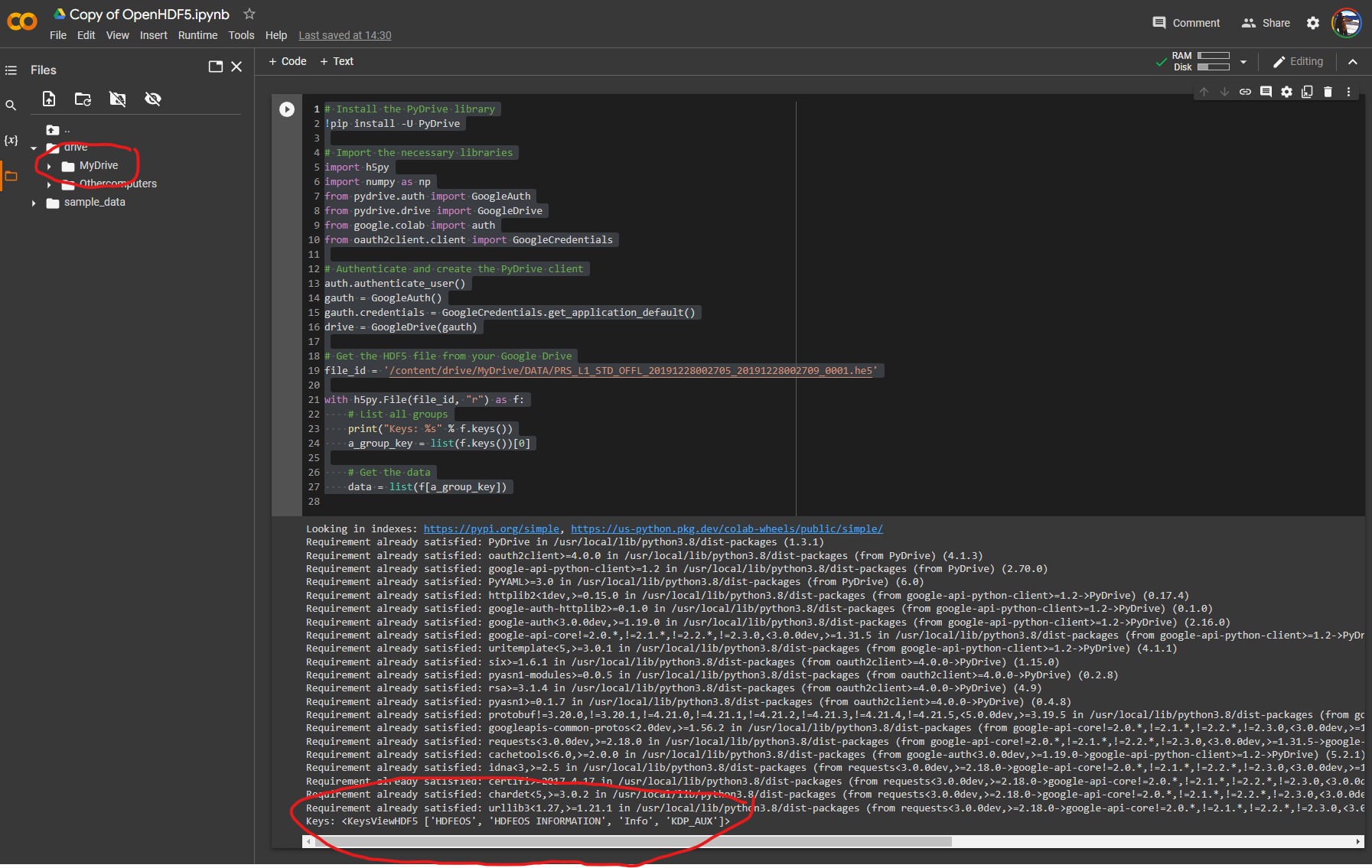
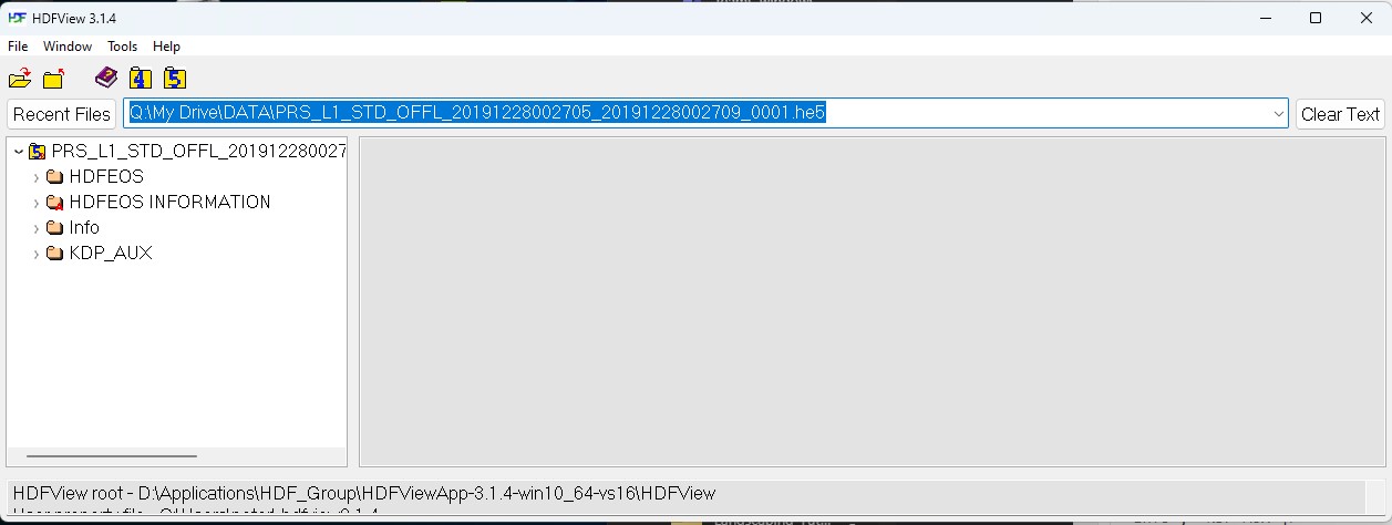
For a first attempt, here is a google colab script for looking at some Philip Island data from the XXX Satellite:
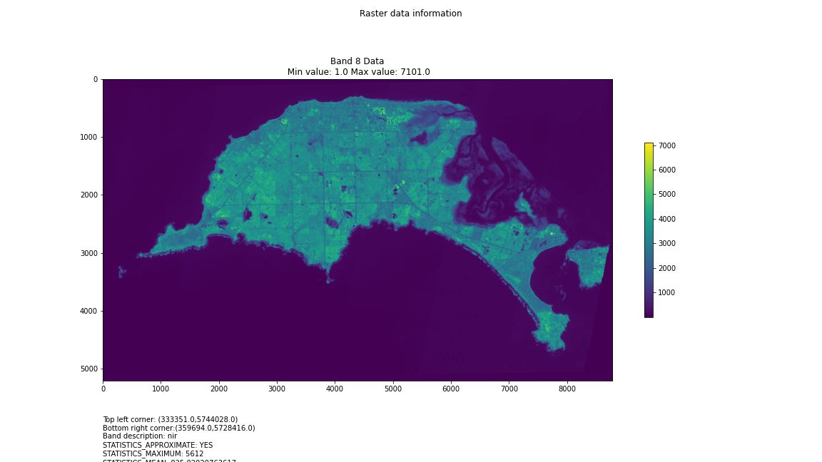
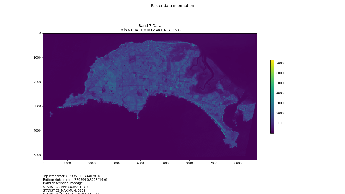
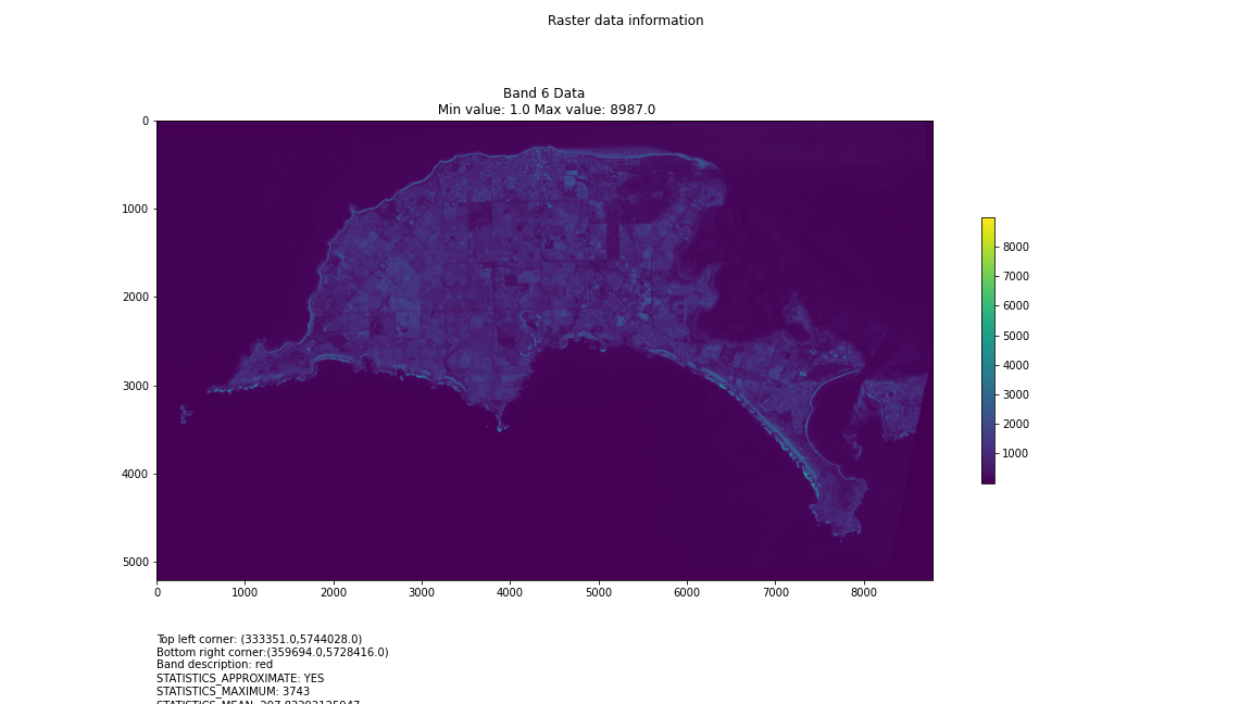
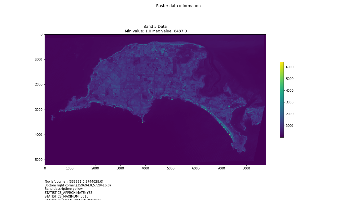
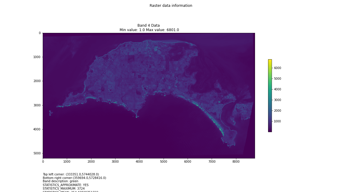
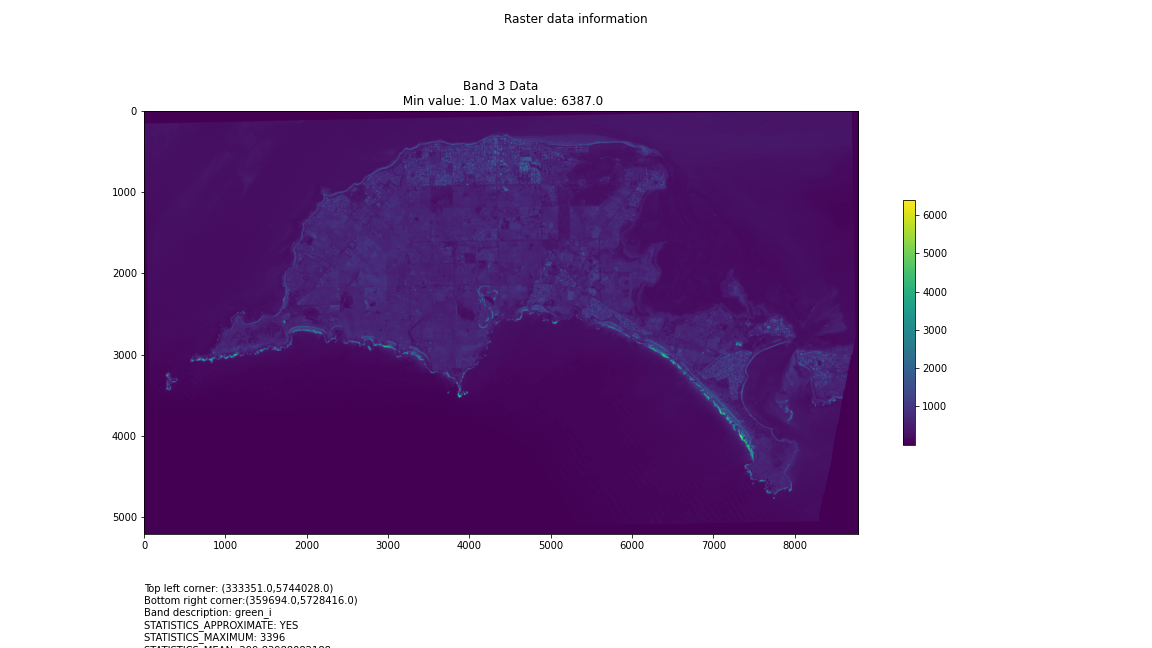
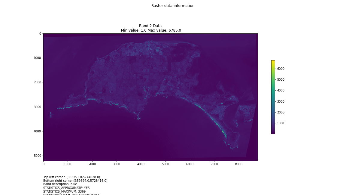
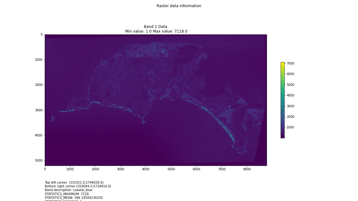
# Import necessary libraries
import os
from osgeo import gdal, gdal_array
from google.colab import drive
import numpy as np
import matplotlib.pyplot as plt
# Mount Google Drive
drive.mount('/content/drive')
#this will ask for permissions - you will need to login through your google account in a pop-up window
# Open the multispectral GeoTIFF file
#set the file path to the folder with the relevant data in it on your google drive (mount this first via the panel to the left of this one - it is called 'drive' and appears as a folder)
file_path = '/content/drive/MyDrive/DATA/XXX_multispectral.tif'
#set a variable for your path and the file you open
src_ds = gdal.Open(file_path)
#use gdal to get some characteristics of the data in the file
print("Projection: ", src_ds.GetProjection())  # get projection
print("Columns:", src_ds.RasterXSize)  # number of columns
print("Rows:", src_ds.RasterYSize)  # number of rows
print("Band count:", src_ds.RasterCount)  # number of bands
print("GeoTransform", src_ds.GetGeoTransform()) #affine transform
# Use gdalinfo command to print and save information about the raster file - this is extracted from the geotiff itself
info = gdal.Info(file_path)
print(info)
if not os.path.exists("/content/drive/MyDrive/DATA/OUTPUT"):
    os.makedirs("/content/drive/MyDrive/DATA/OUTPUT")
info_file = os.path.join("/content/drive/MyDrive/DATA/OUTPUT", "raster_info.txt")
with open(info_file, "w") as f:
    f.write(info)
# Retrieve the band count and band metadata
data_array = src_ds.GetRasterBand(1).ReadAsArray()
data_array.shape
band_count = src_ds.RasterCount
# Loop through each band and display in a matplotlib image
for i in range(1, band_count+1):
    band = src_ds.GetRasterBand(i)
    minval, maxval = band.ComputeRasterMinMax()
    data_array = band.ReadAsArray()
    plt.figure(figsize=(16, 9))
    plt.imshow(data_array, vmin=minval, vmax=maxval)
    plt.colorbar(anchor=(0, 0.3), shrink=0.5)
    plt.title("Band {} Data\n Min value: {} Max value: {}".format(i, minval, maxval))
    plt.suptitle("Raster data information")
    band_description = band.GetDescription()
    metadata = band.GetMetadata_Dict()
    geotransform = src_ds.GetGeoTransform()
    top_left_x = geotransform[0]
    top_left_y = geotransform[3]
    w_e_pixel_res = geotransform[1]
    n_s_pixel_res = geotransform[5]
    x_size = src_ds.RasterXSize
    y_size = src_ds.RasterYSize
    bottom_right_x = top_left_x + (w_e_pixel_res * x_size)
    bottom_right_y = top_left_y + (n_s_pixel_res * y_size)
    coordinates = ["Top left corner: ({},{})".format(top_left_x,top_left_y),"Bottom right corner:({},{})".format(bottom_right_x,bottom_right_y)]
    if band_description:
        metadata_list = ["Band description: {}".format(band_description)]
    else:
        metadata_list = ["Band description is not available"]
    if metadata:
        metadata_list += ["{}: {}".format(k, v) for k, v in metadata.items()]
    else:
        metadata_list += ["Metadata is not available"]
    plt.annotate("\n".join(coordinates+metadata_list), (0,0), (0, -50), xycoords='axes fraction', textcoords='offset points', va='top')
    plt.savefig("/content/drive/MyDrive/DATA/OUTPUT/Band_{}_Data.png".format(i), vmin=minval, vmax=maxval)
    plt.show()


This works well enough for a plot – but it’s interesting (a debate) – whether it is best/easiest to use GDAL or the rasterio Mapbox wrapper. Tests will tell. And there is Pandas too. They all have pros and cons. Try it yourself and let us know,

I’m looking into ways of sharing the colabs more directly for those who are interested – that’s the whole point.

Visualising Satellite data using Google Colab

Having spent a few hours reading documentation and having an ongoing conversation with chatGPT, I’m getting the hang of the hdf5 file structure and can now visualise some multispectral data in Google Colab:


from google.colab import drive
drive.mount('/content/drive')

import h5py
import numpy as np
import matplotlib.pyplot as plt

# Get the HDF5 file from your Google Drive
file_id = '/content/drive/MyDrive/DATA/file_name.he5'

with h5py.File(file_id, "r") as f:
# List all groups
print("Keys: %s" % f.keys())
a_group_key = list(f.keys())[0]

# Get the data
data = list(f[a_group_key])

#This gives us some idea about the groups/keys in the hdf file and some idea about the datasets contained therein - but will become more detailed as we go along

# Open the HDF5 file
with h5py.File(file_id, 'r') as f:
# Open the data field
#currently this is hard-coded as I know from hdfView that this is the path I want to look at - but really we want to find this programmatically.
data_field = f['/path_to/Data Fields/Cube']
# Print the shape of the data field
print(f'Shape: {data_field.attrs}')
print(f'Shape: {data_field.dtype}')
print(f'Shape: {data_field.shape}')
#This gives us some idea about the data cube we are examining - such as its attributes, data type and shape (typically rows and columns) - it'll print them to output

# Open the HDF5 file
with h5py.File(file_id, 'r') as f:
# Open the data field
data_field = f['/path_to/Data Fields/Cube']
# Get the data and reshape it to 2D
data = np.array(data_field[:]).reshape(data_field.shape[0], data_field.shape[1])
# Scale the data to fit within an 800x800 pixels
data = np.uint8(np.interp(data, (data.min(), data.max()), (0, 255)))
# Create a figure with the specified size
fig = plt.figure(figsize=(8, 8))
# Add the data to the figure
plt.imshow(data, cmap='viridis')
# Display the figure
plt.show()

Satellite data plotted with viridis colourmap

Next steps involve developing a way of iteratively traversing the hdf5 directory structure, so that I can identify relevant data fields within the file – they’re not explicitly identified as ‘image files’. This can be done using h5py functions. Another thing to explore is GDAL: once I’ve identified the correct data in geolocation fields, it should become possible to output geotiffs or UE-friendly png files with geolocation metadata.

Here’s some other matplotlib colourmaps applied to the same dataset.

It’s all pretty crude at this point – just figuring out how this stuff might work.

ChatGPT, Google Colab and Hyperspectral Data

It occurs to me that, rather than going to all the hassle of figuring out how to write all the code for colab myself, that I can use my chatGPT assistant to do it for me:

Q: write a script for google colab to extract images from an hdf5 file located upon my google drive


Chat GPT:

Here is an example script that demonstrates how to extract images from an HDF5 file located on your Google Drive using the h5py library in Python, and the PyDrive library to interact with Google Drive:

# Install the PyDrive library
!pip install -U PyDrive

# Import the necessary libraries
import h5py
import numpy as np
from pydrive.auth import GoogleAuth
from pydrive.drive import GoogleDrive
from google.colab import auth
from oauth2client.client import GoogleCredentials

# Authenticate and create the PyDrive client
auth.authenticate_user()
gauth = GoogleAuth()
gauth.credentials = GoogleCredentials.get_application_default()
drive = GoogleDrive(gauth)

# Get the HDF5 file from your Google Drive
file_id = '<YOUR FILE ID>'
downloaded = drive.CreateFile({'id': file_id})
downloaded.GetContentFile('hyperspectral_image_data.hdf5')

# Open the HDF5 file
with h5py.File('hyperspectral_image_data.hdf5', 'r') as hdf5_file:
# Access the dataset containing the images
images = hdf5_file['images']
# Extract an image by its index
image = np.array(images[0])
print(image)

Make sure to replace <YOUR FILE ID> with the actual file ID of the HDF5 file on your Google Drive. You can find the file ID by opening the file in Google Drive and looking at the URL – the file ID is the string of letters and numbers after the last forward slash.

You can also use the gdal_translate command with the PyDrive library as well, just add the following lines of code to download the file and then use gdal_translate command to convert to tiff or geotiff

# Get the HDF5 file from your Google Drive
file_id = '<YOUR FILE ID>'
downloaded = drive.CreateFile({'id': file_id})
downloaded.GetContentFile('hyperspectral_image_data.hdf ')#Use gdal_translate
!gdal_translate -of GTiff HDF5:"hyperspectral_image_data.hdf5"://dataset output.tif

You can then use any image processing library to open and read the image.


Lots of interesting things to unpack in this advice – and lots of errors as I expect to debug the code.

So, as a first step, let’s see if we can just get access to the file and some basic metadata.

# Install the PyDrive library
!pip install -U PyDrive
# Import the necessary libraries
import h5py
import numpy as np
from pydrive.auth import GoogleAuth
from pydrive.drive import GoogleDrive
from google.colab import auth
from oauth2client.client import GoogleCredentials
# Authenticate and create the PyDrive client
auth.authenticate_user()
gauth = GoogleAuth()
gauth.credentials = GoogleCredentials.get_application_default()
drive = GoogleDrive(gauth)
# Get the HDF5 file from your Google Drive
file_id = '/content/drive/MyDrive/DATA/XXXXXXX.he5'
with h5py.File(file_id, "r") as f:
    # List all groups
    print("Keys: %s" % f.keys())
    a_group_key = list(f.keys())[0]
    # Get the data
    data = list(f[a_group_key])


Success! We can see the HDF keys returned below:

Keys: <KeysViewHDF5 ['HDFEOS', 'HDFEOS INFORMATION', 'Info', 'KDP_AUX']>

These match the top-level directory structure revealed by HDFView:

This is the first step in identifying the file contents, before we can drill down into the file structure to identify a whole bunch of parameters about the datacube that we can do interesting things with 🙂